Subscribe
Alert Me when new Data Products are available


Comparing census demographics from different census years can be a difficult task due to changing geographic boundaries. Our normalized data product line assists researchers with comparisons of data across time by adjusting and weighting the census data to account for changes in geographies.
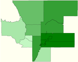
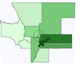
If you are working at the state level then there are no changes. But at all smaller geographies there are changes, some of them quiet dramatic some relatively modest. So for example in Colorado between 2000 and 2010 a new county was added – Broomfield. The surrounding 4 counties each spun off a small piece and created this new county (inside the circle on the 2010 map below).
| Map of 2000 Colorado Counties | Map of 2010 Colorado Counties |
 |
 |
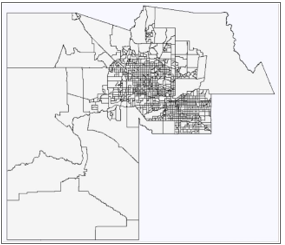
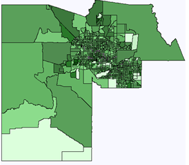
To demonstrate some of the issues associated with changing boundaries, below is a comparison of Maricopa County, Arizona in 2020 and 2010 at the Census Tract level. During this time span, Maricopa County expanded its population going from 3,817,117 to 4,420,568– a 15.8% increase. A quick appraisal of the two maps below demonstrates the numerous changes that occurred in the census tract boundaries, specifically the addition of 93 new tracts in 2010 – a 10% increase..
| 2020 Maricopa County, AZTotal Census Tracts (1009) | 2010 Maricopa County, AZTotal Census Tracts (916) |
 |
 |
While many of these changes were in the most populated central part the outlying areas are the easiest to see these dramatic changes. Here is a zoomed in view of tracts 506.XX and 507.XX
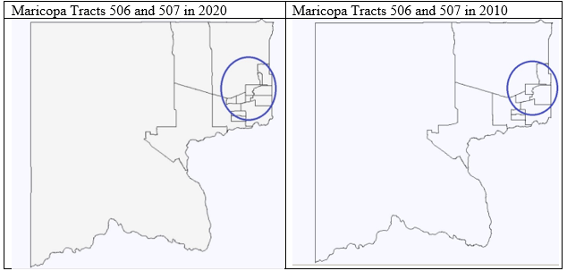 |
In 2010 there were only 11 Tracts as opposed to 16 in 2020 (a 45% increase). The population in these tracts went from 62,196 to 101,334 (a 63% increase). You can see that you could probably do this manually since most of the time the 2 tracts in 2020 could be added together to equal the 1 tract in 2010. But it requires a tremendous amount of work to do this for anything other than a very local region.
The Census’ 2010 American Community Survey is the most complete source of detailed information about the people, housing, and economy of the United States in 2010. This dataset contains variables such as income, housing, employment, language spoken, ancestry, education, poverty, rent, mortgage, commute to work, etc. There are 5,500 variables at the Block Group level and over 16,000 variables at the larger geographies such as tract, zip code, county and state level.
The 2010 American Community Survey in 2020 Boundaries, like all of our census-based products, comes with built-in data viewing and exporting capabilities as well as thematically shaded, color-mapping capabilities. With a few quick keystrokes you can generate full-blown maps or tables. You can extract data as dbf, csv, or shape files and use them as input files for other programs e.g. statistical (SAS, SPSS), database (Access, Oracle), spreadsheet (Excel, 1-2-3), and mapping (Arc View). You can even export any of the geographic boundaries into the mapping packages.
The 2010 American Community Survey lets you easily explore, analyze, and visualize an enormous amount of details about the people, housing, industry, economy, and places in the United States – and once it is put into the 2020 boundaries it makes it simple to compare to the changes from the 2020 Demographics and Housing Characteristics (DHC) or the 2020 American Community Survey for an easy apples-to-apples comparison of the population of the United States.
| Name | Value |
|---|---|
| State User | $695.00 |
| National User | $1295.00 |
| American Community Survey Variables | ✪ 813 tables |
The American Community Survey 2006-2010 was the first data set in the 2010 boundaries but the US Census Bureau was unable to release it at the Zip Code Tabulation Area. That didn’t happen until the ACS 2007-2011. Thus we have created two ACS products in 2020 Boundaries. The ACS 2010 in 2020 Boundaries has the advantage of being 2010. But if you want Zip Code Tabulation Areas then you need to select the ACS 2011 in 2020 Boundaries.
In both instances you will have access data at the following geographic levels (numbers indicate how many specific areas are within that geographic level):
The ACS 2011 in 2020 Boundaries also includes